Aula 5

2 testes de normalidade Shapiro e Bartllet

Carrega dados

library(tidyverse)

Warning: pacote 'tidyverse' foi compilado no R versão 4.4.3

Warning: pacote 'ggplot2' foi compilado no R versão 4.4.3

Warning: pacote 'tibble' foi compilado no R versão 4.4.3

Warning: pacote 'tidyr' foi compilado no R versão 4.4.3

Warning: pacote 'readr' foi compilado no R versão 4.4.3

Warning: pacote 'purrr' foi compilado no R versão 4.4.3

Warning: pacote 'dplyr' foi compilado no R versão 4.4.3

Warning: pacote 'stringr' foi compilado no R versão 4.4.3

Warning: pacote 'forcats' foi compilado no R versão 4.4.3

Warning: pacote 'lubridate' foi compilado no R versão 4.4.3

── Attaching core tidyverse packages ──────────────────────── tidyverse 2.0.0 ──
✔ dplyr     1.2.0     ✔ readr     2.2.0
✔ forcats   1.0.1     ✔ stringr   1.6.0
✔ ggplot2   4.0.2     ✔ tibble    3.3.1
✔ lubridate 1.9.5     ✔ tidyr     1.3.2
✔ purrr     1.2.1     
── Conflicts ────────────────────────────────────────── tidyverse_conflicts() ──
✖ dplyr::filter() masks stats::filter()
✖ dplyr::lag()    masks stats::lag()
ℹ Use the conflicted package (<http://conflicted.r-lib.org/>) to force all conflicts to become errors

insetos <- InsectSprays
insetos |> ggplot (aes(spray, count)) + geom_boxplot(outlier.colour = NA) + geom_jitter (width = 0.1)

##MODELO DE ANOVA

m1 <- lm(count~spray, data = insetos)
m1

Call:
lm(formula = count ~ spray, data = insetos)

Coefficients:
(Intercept)       sprayB       sprayC       sprayD       sprayE       sprayF  
    14.5000       0.8333     -12.4167      -9.5833     -11.0000       2.1667  

summary(m1)

Call:
lm(formula = count ~ spray, data = insetos)

Residuals:
   Min     1Q Median     3Q    Max 
-8.333 -1.958 -0.500  1.667  9.333 

Coefficients:
            Estimate Std. Error t value Pr(>|t|)    
(Intercept)  14.5000     1.1322  12.807  < 2e-16 ***
sprayB        0.8333     1.6011   0.520    0.604    
sprayC      -12.4167     1.6011  -7.755 7.27e-11 ***
sprayD       -9.5833     1.6011  -5.985 9.82e-08 ***
sprayE      -11.0000     1.6011  -6.870 2.75e-09 ***
sprayF        2.1667     1.6011   1.353    0.181    
---
Signif. codes:  0 '***' 0.001 '**' 0.01 '*' 0.05 '.' 0.1 ' ' 1

Residual standard error: 3.922 on 66 degrees of freedom
Multiple R-squared:  0.7244,    Adjusted R-squared:  0.7036 
F-statistic:  34.7 on 5 and 66 DF,  p-value: < 2.2e-16

anova(m1)

Analysis of Variance Table

Response: count
          Df Sum Sq Mean Sq F value    Pr(>F)    
spray      5 2668.8  533.77  34.702 < 2.2e-16 ***
Residuals 66 1015.2   15.38                      
---
Signif. codes:  0 '***' 0.001 '**' 0.01 '*' 0.05 '.' 0.1 ' ' 1

hist(m1$residuals)

shapiro.test(m1$residuals)

    Shapiro-Wilk normality test

data:  m1$residuals
W = 0.96006, p-value = 0.02226

bartlett.test(count~spray, data = insetos)

    Bartlett test of homogeneity of variances

data:  count by spray
Bartlett's K-squared = 25.96, df = 5, p-value = 9.085e-05

library(performance)

Warning: pacote 'performance' foi compilado no R versão 4.4.3

check_normality(m1)

Warning: Non-normality of residuals detected (p = 0.022).

check_heteroscedasticity(m1)

Warning: Heteroscedasticity (non-constant error variance) detected (p < .001).

##dessa forma vamos usar o teste não paramétrico

kruskal.test(count~spray, data = insetos)

    Kruskal-Wallis rank sum test

data:  count by spray
Kruskal-Wallis chi-squared = 54.691, df = 5, p-value = 1.511e-10

library(DHARMa)

Warning: pacote 'DHARMa' foi compilado no R versão 4.4.3

This is DHARMa 0.4.7. For overview type '?DHARMa'. For recent changes, type news(package = 'DHARMa')

plot(simulateResiduals(m1))

insetos2 <- insetos |> mutate(count2 = sqrt (count))
insetos2

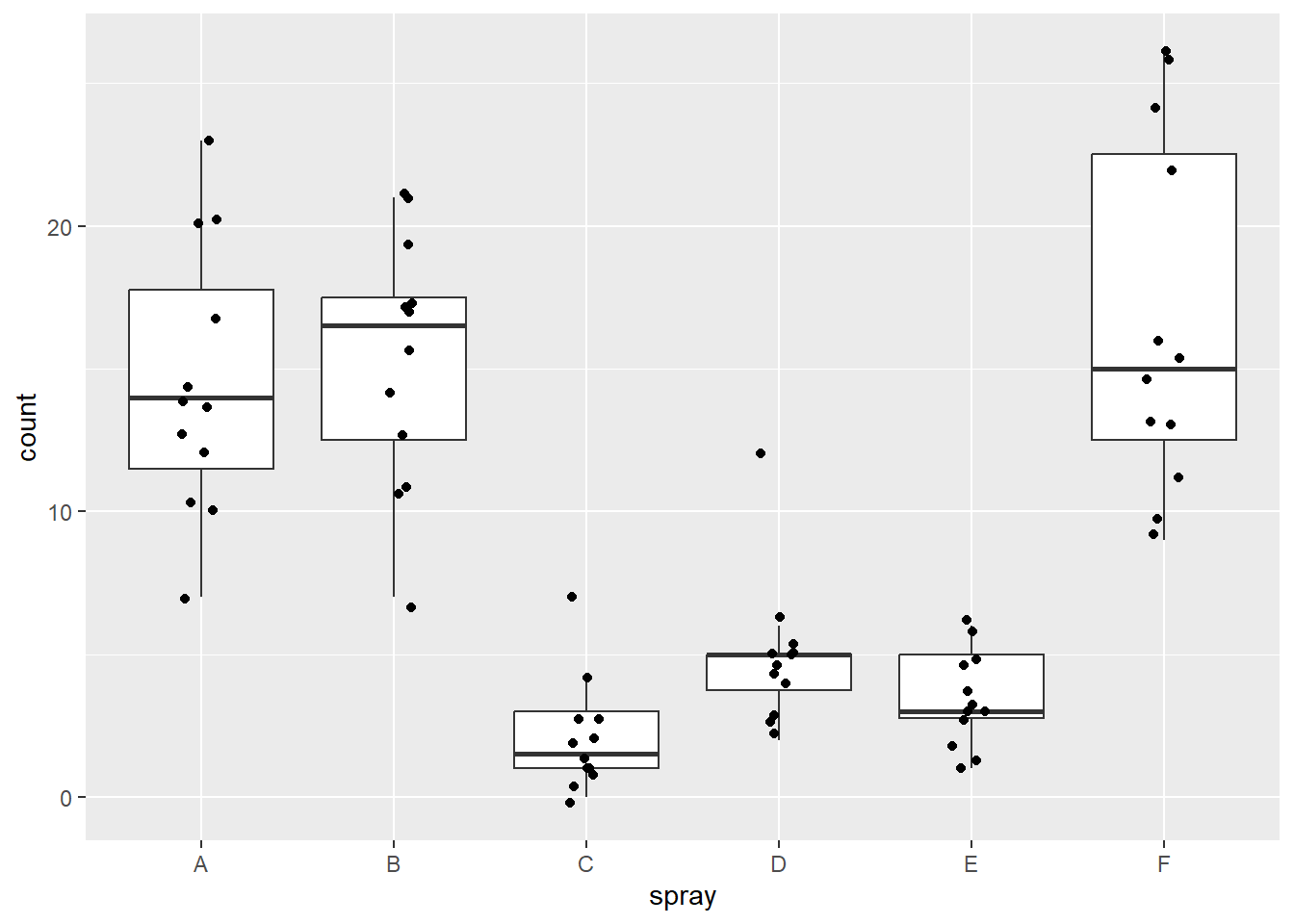
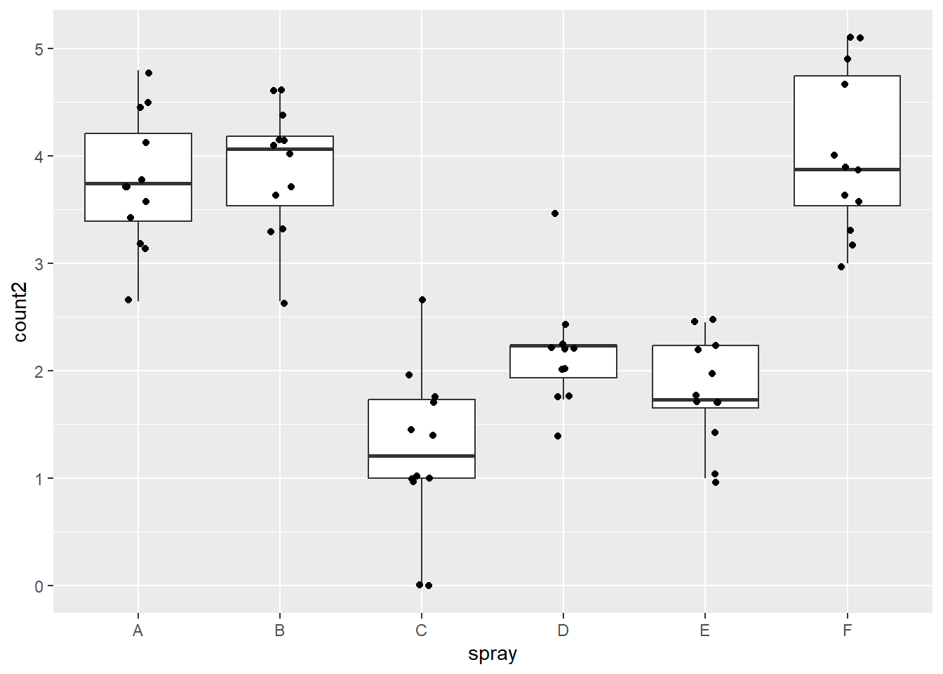
   count spray   count2
1     10     A 3.162278
2      7     A 2.645751
3     20     A 4.472136
4     14     A 3.741657
5     14     A 3.741657
6     12     A 3.464102
7     10     A 3.162278
8     23     A 4.795832
9     17     A 4.123106
10    20     A 4.472136
11    14     A 3.741657
12    13     A 3.605551
13    11     B 3.316625
14    17     B 4.123106
15    21     B 4.582576
16    11     B 3.316625
17    16     B 4.000000
18    14     B 3.741657
19    17     B 4.123106
20    17     B 4.123106
21    19     B 4.358899
22    21     B 4.582576
23     7     B 2.645751
24    13     B 3.605551
25     0     C 0.000000
26     1     C 1.000000
27     7     C 2.645751
28     2     C 1.414214
29     3     C 1.732051
30     1     C 1.000000
31     2     C 1.414214
32     1     C 1.000000
33     3     C 1.732051
34     0     C 0.000000
35     1     C 1.000000
36     4     C 2.000000
37     3     D 1.732051
38     5     D 2.236068
39    12     D 3.464102
40     6     D 2.449490
41     4     D 2.000000
42     3     D 1.732051
43     5     D 2.236068
44     5     D 2.236068
45     5     D 2.236068
46     5     D 2.236068
47     2     D 1.414214
48     4     D 2.000000
49     3     E 1.732051
50     5     E 2.236068
51     3     E 1.732051
52     5     E 2.236068
53     3     E 1.732051
54     6     E 2.449490
55     1     E 1.000000
56     1     E 1.000000
57     3     E 1.732051
58     2     E 1.414214
59     6     E 2.449490
60     4     E 2.000000
61    11     F 3.316625
62     9     F 3.000000
63    15     F 3.872983
64    22     F 4.690416
65    15     F 3.872983
66    16     F 4.000000
67    13     F 3.605551
68    10     F 3.162278
69    26     F 5.099020
70    26     F 5.099020
71    24     F 4.898979
72    13     F 3.605551

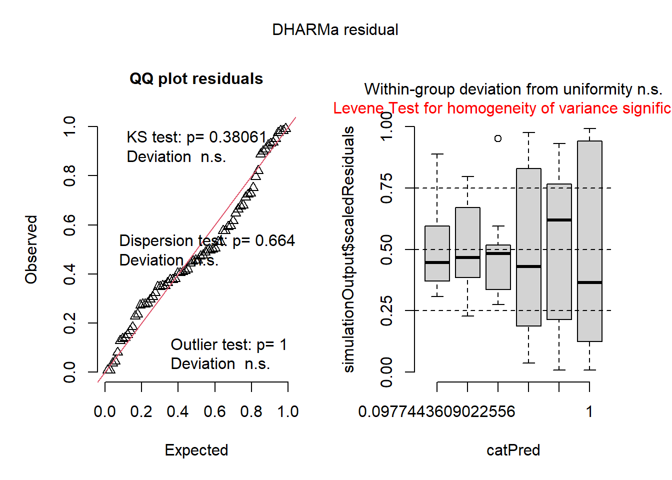
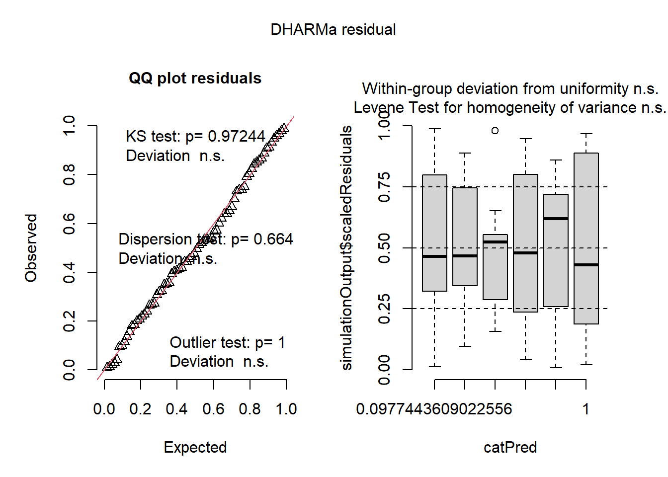
##agora o modelo resposta será o count2

m2 <- lm(sqrt (count) ~spray, data = insetos2)
m2

Call:
lm(formula = sqrt(count) ~ spray, data = insetos2)

Coefficients:
(Intercept)       sprayB       sprayC       sprayD       sprayE       sprayF  
     3.7607       0.1160      -2.5158      -1.5963      -1.9512       0.2579  

summary(m2)

Call:
lm(formula = sqrt(count) ~ spray, data = insetos2)

Residuals:
     Min       1Q   Median       3Q      Max 
-1.24486 -0.39970 -0.01902  0.42661  1.40089 

Coefficients:
            Estimate Std. Error t value Pr(>|t|)    
(Intercept)   3.7607     0.1814  20.733  < 2e-16 ***
sprayB        0.1160     0.2565   0.452    0.653    
sprayC       -2.5158     0.2565  -9.807 1.64e-14 ***
sprayD       -1.5963     0.2565  -6.223 3.80e-08 ***
sprayE       -1.9512     0.2565  -7.606 1.34e-10 ***
sprayF        0.2579     0.2565   1.006    0.318    
---
Signif. codes:  0 '***' 0.001 '**' 0.01 '*' 0.05 '.' 0.1 ' ' 1

Residual standard error: 0.6283 on 66 degrees of freedom
Multiple R-squared:  0.7724,    Adjusted R-squared:  0.7552 
F-statistic:  44.8 on 5 and 66 DF,  p-value: < 2.2e-16

anova(m2)

Analysis of Variance Table

Response: sqrt(count)
          Df Sum Sq Mean Sq F value    Pr(>F)    
spray      5 88.438 17.6876  44.799 < 2.2e-16 ***
Residuals 66 26.058  0.3948                      
---
Signif. codes:  0 '***' 0.001 '**' 0.01 '*' 0.05 '.' 0.1 ' ' 1

hist(m2$residuals)

shapiro.test(m2$residuals)

    Shapiro-Wilk normality test

data:  m2$residuals
W = 0.98721, p-value = 0.6814

bartlett.test(count2~spray, data = insetos2)

    Bartlett test of homogeneity of variances

data:  count2 by spray
Bartlett's K-squared = 3.7525, df = 5, p-value = 0.5856

insetos2 |> ggplot (aes(spray, count2)) + geom_boxplot(outlier.colour = NA) + geom_jitter (width = 0.1)

library(performance)
check_normality(m2)

OK: residuals appear as normally distributed (p = 0.681).

check_heteroscedasticity(m2)

OK: Error variance appears to be homoscedastic (p = 0.854).

library(DHARMa)

plot(simulateResiduals(m2))

library(emmeans)

Warning: pacote 'emmeans' foi compilado no R versão 4.4.3

Welcome to emmeans.
Caution: You lose important information if you filter this package's results.
See '? untidy'

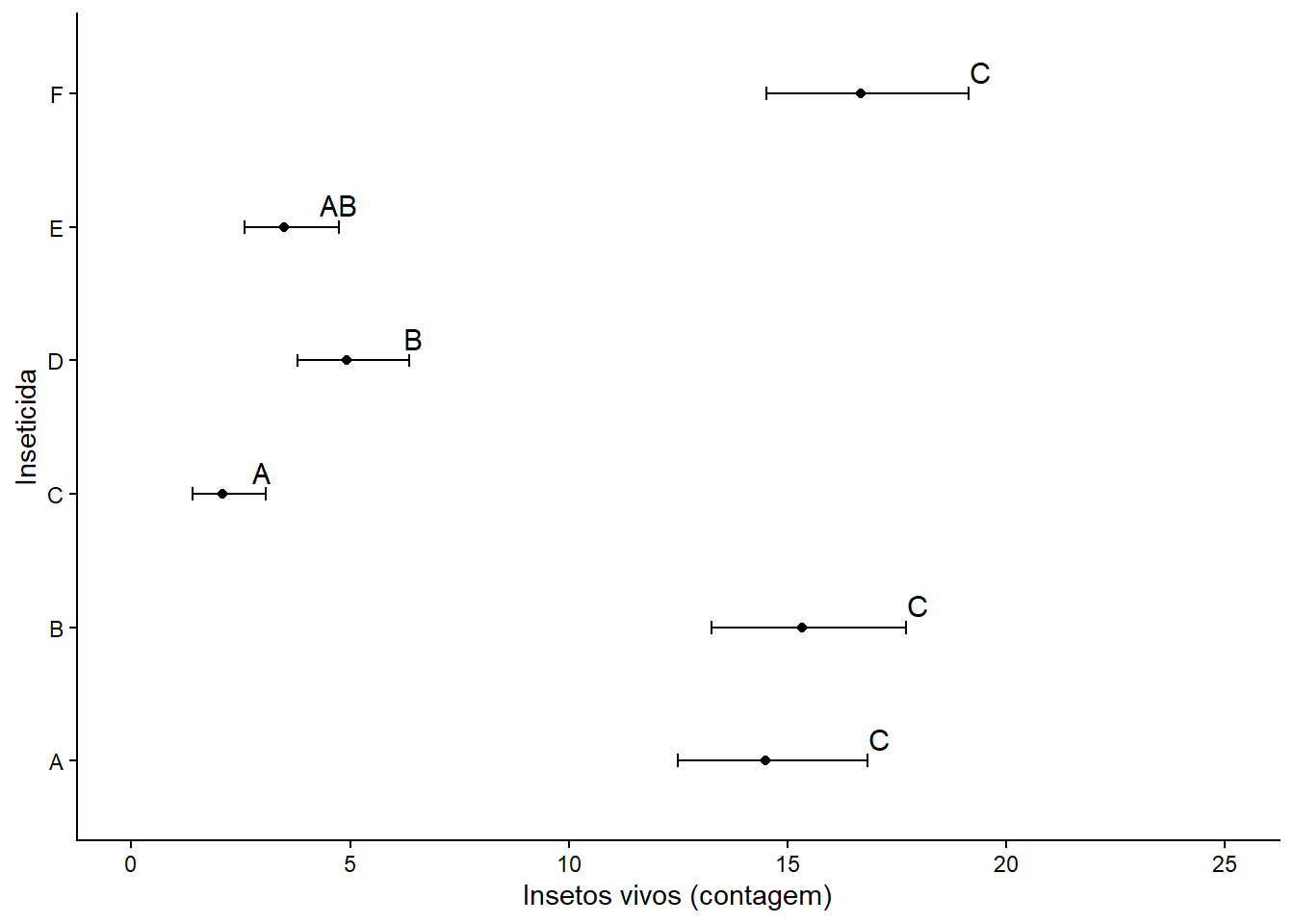
medias2 <- emmeans (m2,~ spray, type  = "response")
medias2

 spray response    SE df lower.CL upper.CL
 A        14.14 1.360 66   11.550    17.00
 B        15.03 1.410 66   12.352    17.97
 C         1.55 0.452 66    0.779     2.58
 D         4.68 0.785 66    3.248     6.38
 E         3.27 0.656 66    2.095     4.72
 F        16.15 1.460 66   13.370    19.19

Confidence level used: 0.95 
Intervals are back-transformed from the sqrt scale 

library(multcomp)

Warning: pacote 'multcomp' foi compilado no R versão 4.4.3

Carregando pacotes exigidos: mvtnorm

Warning: pacote 'mvtnorm' foi compilado no R versão 4.4.3

Carregando pacotes exigidos: survival

Carregando pacotes exigidos: TH.data

Warning: pacote 'TH.data' foi compilado no R versão 4.4.3

Carregando pacotes exigidos: MASS

Anexando pacote: 'MASS'

O seguinte objeto é mascarado por 'package:dplyr':

    select

Anexando pacote: 'TH.data'

O seguinte objeto é mascarado por 'package:MASS':

    geyser

cld(medias2, Letters = LETTERS)

 spray response    SE df lower.CL upper.CL .group
 C         1.55 0.452 66    0.779     2.58  A    
 E         3.27 0.656 66    2.095     4.72  AB   
 D         4.68 0.785 66    3.248     6.38   B   
 A        14.14 1.360 66   11.550    17.00    C  
 B        15.03 1.410 66   12.352    17.97    C  
 F        16.15 1.460 66   13.370    19.19    C  

Confidence level used: 0.95 
Intervals are back-transformed from the sqrt scale 
Note: contrasts are still on the sqrt scale. Consider using
      regrid() if you want contrasts of back-transformed estimates. 
P value adjustment: tukey method for comparing a family of 6 estimates 
significance level used: alpha = 0.05 
NOTE: If two or more means share the same grouping symbol,
      then we cannot show them to be different.
      But we also did not show them to be the same. 

library(agricolae)

Warning: pacote 'agricolae' foi compilado no R versão 4.4.3

k <- kruskal(insetos$count, insetos$spray)
k

$statistics
     Chisq Df      p.chisq  t.value      MSD
  54.69134  5 1.510845e-10 1.996564 8.462804

$parameters
            test p.ajusted        name.t ntr alpha
  Kruskal-Wallis      none insetos$spray   6  0.05

$means
  insetos.count     rank      std  r Min Max   Q25  Q50   Q75
A     14.500000 52.16667 4.719399 12   7  23 11.50 14.0 17.75
B     15.333333 54.83333 4.271115 12   7  21 12.50 16.5 17.50
C      2.083333 11.45833 1.975225 12   0   7  1.00  1.5  3.00
D      4.916667 25.58333 2.503028 12   2  12  3.75  5.0  5.00
E      3.500000 19.33333 1.732051 12   1   6  2.75  3.0  5.00
F     16.666667 55.62500 6.213378 12   9  26 12.50 15.0 22.50

$comparison
NULL

$groups
  insetos$count groups
F      55.62500      a
B      54.83333      a
A      52.16667      a
D      25.58333      b
E      19.33333     bc
C      11.45833      c

attr(,"class")
[1] "group"

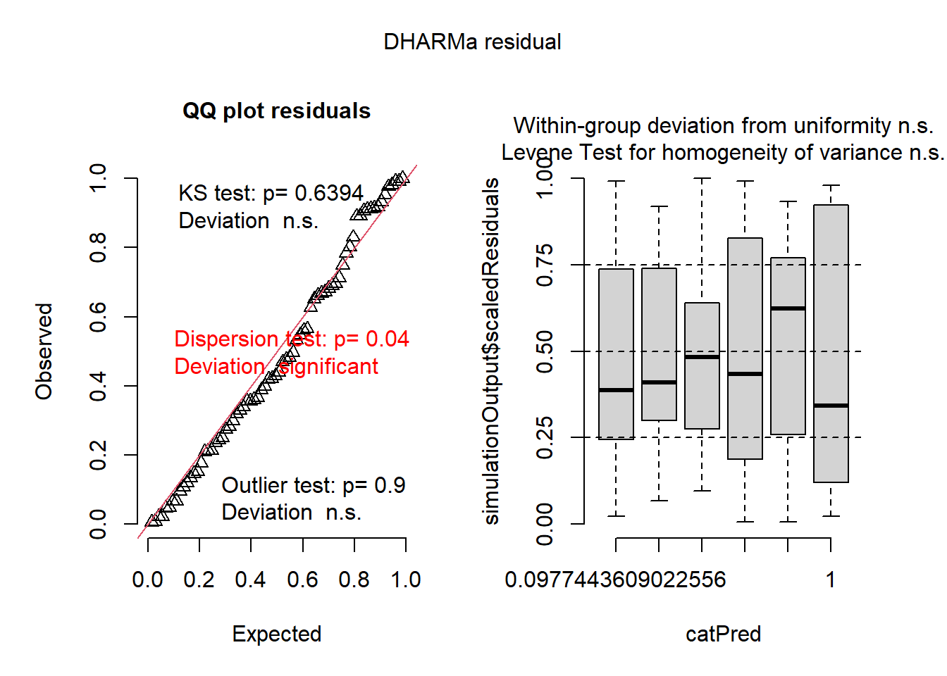
##GLM com A FAMILIA E FUNÇÃO DE LIGAÇÃO

m3 <- glm(count ~ spray, family = poisson(link = "log"), data = insetos)

plot(simulateResiduals(m3))

df3 <- cld(emmeans(m3,~ spray, type = "response"), Letters = LETTERS)

df3 |> 
  ggplot(aes(spray, rate, label = .group)) + geom_point() + geom_errorbar(aes(ymin = asymp.LCL, ymax = asymp.UCL), width = 0.1) + ylim(0, 25) + geom_text(aes(y = asymp.UCL), vjust = -0.5, size = 4) + theme_classic() +
  labs(x = "Inseticida", y = "Insetos vivos (contagem)")+coord_flip()

#o coord_flip inverte o x com o y